Geodesic domes are fascinating structures that can span over large spaces without the need for extensive support or a significant amount of materials. But, how do you go about building one? While you can find plenty of guides that explain the process using chord length and similar techniques, they often lack an explanation of the fundamental principles. This limitation can restrict your options when you want to deviate from or adapt the dome’s shape to meet specific constraints.

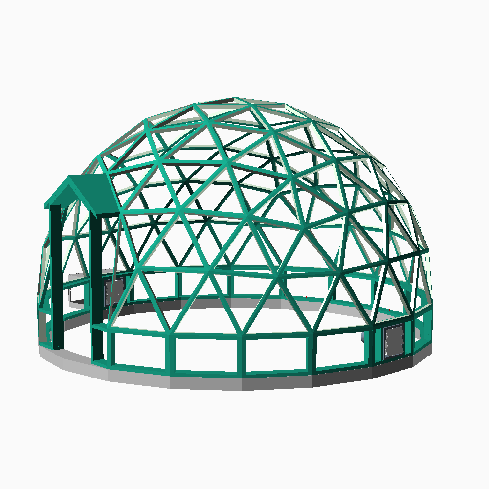
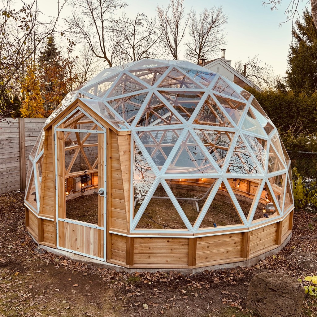
A popular DIY project for enthusiasts like myself is building a greenhouse dome. It offers a remarkable opportunity to engage in a fun and practical activity simultaneously.

Having the ability to model the greenhouse using OpenSCAD proved to be quite valuable, especially when designing customized triangles to fit the door. Before we dive into the OpenSCAD source code, let’s begin with a brief overview of the model. The geodesic dome is constructed based on a convex regular icosahedron, consisting of 20 identical equilateral triangles. The concept involves subdividing these icosahedron faces into smaller triangles and projecting them onto the circumscribing sphere.

The initial step in creating an OpenSCAD geodesic dome is to construct a convex regular icosahedron. This process begins with defining the Cartesian coordinates of the 12 vertices.

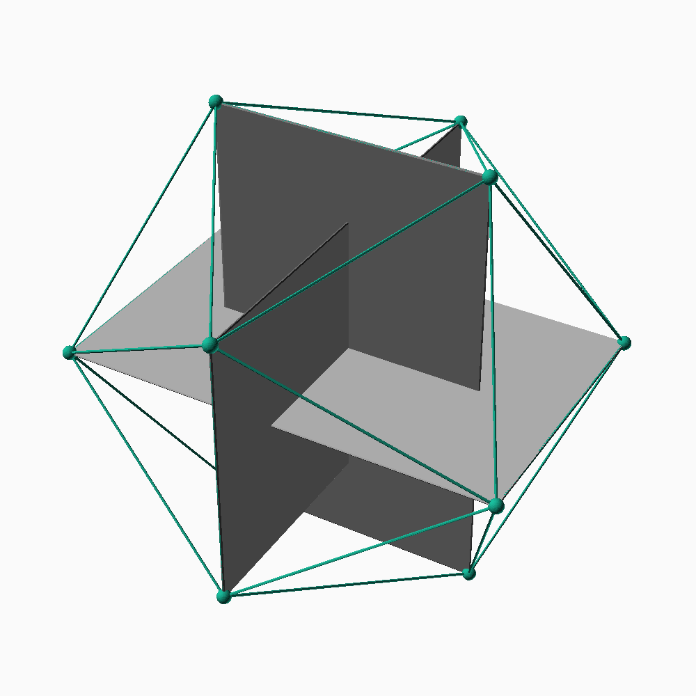
The coordinates are (±phi,±1,0), (±1,0,±phi) and (0,±phi,±1)

where phi = (1+√5)/2 is the golden ratio.

Copy and paste the code below to create an icosahedron in OpenSCAD.

PHI = (1+sqrt(5))/2;

icosahedron_vertices =
[
    [-PHI,-1,0], [-1,0,-PHI], [0,-PHI,-1],
    [ PHI,-1,0], [ 1,0,-PHI], [0, PHI,-1],
    [-PHI, 1,0], [-1,0, PHI], [0,-PHI, 1],
    [ PHI, 1,0], [ 1,0, PHI], [0, PHI, 1]
];


icosahedron_faces = // made of 20 triangles
[ 
    [ 1, 0, 2],
    [ 1, 2, 4],
    [ 1, 4, 5],
    [ 1, 5, 6],
    [ 1, 6, 0],
    [10, 3, 8],
    [10, 8, 7],
    [10, 7,11],
    [10,11, 9],
    [10, 9, 3],
    [ 8, 2, 0],
    [ 8, 0, 7],
    [ 7, 0, 6],
    [ 7, 6,11],
    [11, 6, 5],
    [11, 5, 9],
    [ 9, 5, 4],
    [ 9, 4, 3],
    [ 3, 4, 2],
    [ 3, 2, 8]
];

polyhedron(icosahedron_vertices, icosahedron_faces);

Now that we have the fundamental shape modeled in OpenSCAD, we need to divide each face into multiple triangles. For example, a frequency 4 dome contains 16 triangles (4 times 4) on each face of the icosahedron.

There are many ways to achieve this, but here we will simply begin by dividing the icosahedron face into 4 equilateral triangles, and then each of these triangles will be further subdivided into 4, resulting in a total of 16 equilateral triangles.

function middle_point(p1,p2) = 
    [ (p1.x+p2.x)/2, (p1.y+p2.y)/2, (p1.z+p2.z)/2 ];

// Split Triangle F2
//  - Split a triangle into four triangles
//
//             *p1                         *p1
//            * *                         * *
//           *   *            \          *   *
//          *     *            \        *     *
//         *       *     -------+   p31* * * * *p12
//        *         *          /      * *     * *
//       *           *        /      *   *   *   *
//      *             *             *     * *     *
//   p3* * * * * * * * *p2       p3* * * * * * * * *p2
//                                         p23
function split_triangle_f2(triangle) =
    let (p1 = triangle[0], p2 = triangle[1], p3 = triangle[2])
    let (p12 = middle_point(p1,p2))
    let (p23 = middle_point(p2,p3))
    let (p31 = middle_point(p3,p1))
    [ [p1,p12,p31],[p2,p23,p12],[p3,p31,p23],[p12,p23,p31] ];

// Split Triangle F4
//  - Split a triangle into 16 triangles
function split_triangle_f4(triangle) =
    let (f2 = split_triangle_f2(triangle))
    concat(split_triangle_f2(f2[0]), 
           split_triangle_f2(f2[1]), 
           split_triangle_f2(f2[2]), 
           split_triangle_f2(f2[3]));

The triangles must be projected onto the circumscribing sphere.

To simplify this step, we will use spherical coordinates. Once a point in space is expressed in spherical coordinates, projecting it onto the sphere is as simple as adjusting its radial distance to the desired value. To proceed in this manner, we need functions for converting between the Cartesian and spherical reference systems.

// In the spherical coordiate system, a point P in space is
// represented by the ordered triple (ρ,θ,φ) where
//   ρ  rho    distance between P the origin O
//   θ  theta  is the angle formed by the positive x-axis
//             and the line segment OP projected on the xy
//             plane
//   φ  phi    is the angle formed by the positive z-axis
//             and the line segment OP (0 ≤ φ ≤ π)

// convert from spherical to rectangular coordinates
//   x = ρ sin φ cos θ
//   y = ρ sin φ sin θ
//   z = ρ cos φ
function to_rectangular(p  /*[rho,theta,phi]*/) =
    let (rho = p[0])
    [ rho*sin(p[2])*cos(p[1]),
      rho*sin(p[2])*sin(p[1]),
      rho*cos(p[2]) ];

// convert from rectangular to spherical coordinates
//   ρ = sqrt( x^2 + y^2 + z^2 )
//   θ = arctan( y/x )
//   φ = arccos( z/ρ )
function to_spherical(p /*[x,y,z]*/) = 
    let (rho = sqrt(p.x^2 + p.y^2 + p.z^2))
    p.x==0 && p.y==0 ? p.z<0 ? [-p.z,0,180] : [p.z,0,0] : 
    [ rho,
      p.x>=0 ? atan(p.y/p.x) : 180 + atan(p.y/p.x),
      acos(p.z/rho) ];

With these functions at our disposal, we can now easily project onto a sphere.

// Input:
//   p point in rectangular coordinates (x,y,z)
//   r radius of the sphere
// Output:
//   point in rectangular coordinates (x2,y2,z2)
// This function converts p into spherical coordinates and change
// its radius to r and convert back into rectangular coordinates
function project_point_on_sphere(p,r) =
    let (s = to_spherical(p))
    to_rectangular([r,s[1],s[2]]);

// Same as project_point_on_sphere, but applies to a triangle
function project_triangle_on_sphere(triangle, r) =
    let (s1 = to_spherical(triangle[0]))
    let (s2 = to_spherical(triangle[1]))
    let (s3 = to_spherical(triangle[2]))
    [ to_rectangular([r,s1[1],s1[2]]),
      to_rectangular([r,s2[1],s2[2]]),
      to_rectangular([r,s3[1],s3[2]]) ];

At this point, we have all the necessary tools to create a frequency 4 geodesic sphere. However, what we currently possess is a vector containing numerous triangles expressed in Cartesian coordinates. In the next step within OpenSCAD, we need to ‘draw’ these triangles. OpenSCAD is capable of handling 3D shapes, so we require a module that takes a triangle as input and generates a 3D volume as the output.

module panel(triangle, inner_radius, outer_radius)
{
    inner_triangle = project_triangle_on_sphere(triangle,inner_radius);
    outer_triangle = project_triangle_on_sphere(triangle,outer_radius);
    polyhedron(
        concat(outer_triangle,inner_triangle), 
        [[0,1,2], [0,3,4,1], [1,4,5,2], [2,5,3,0], [3,5,4]]);    
}

We can render the entire frequency 4 geodesic sphere by iterating through all the icosahedron faces.

for (i=[0:len(icosahedron_faces)-1])
    for (t=icosahedron_f4_triangles(i))
        panel(t, 29,30);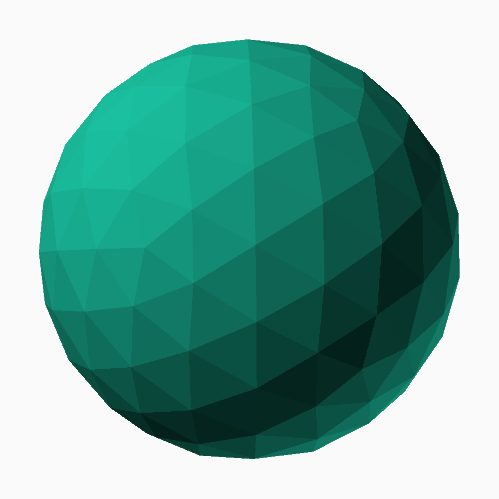

For a dome, we render only the triangles above the equator. However, this reveals that the triangles at the equator are not flat on it.

function triangle_above_equator(triangle) =
    triangle[0].z >= 0 && 
    triangle[1].z >= 0 && 
    triangle[2].z >= 0;

for (i=[0:len(icosahedron_faces)-1])
    for (t=icosahedron_f4_triangles(i))
        if (triangle_above_equator(t))
            panel(t, 29,30);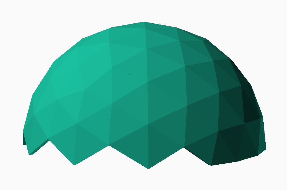

To resolve this issue, we rotate the sphere to an angle where all the triangles align properly. Since everything is based on the icosahedron, rotating it and applying all subsequent transformations will result in the desired geodesic sphere.

original_icosahedron_vertices =
[
    [-PHI,-1,0], [-1,0,-PHI], [0,-PHI,-1],
    [ PHI,-1,0], [ 1,0,-PHI], [0, PHI,-1],
    [-PHI, 1,0], [-1,0, PHI], [0,-PHI, 1],
    [ PHI, 1,0], [ 1,0, PHI], [0, PHI, 1]
];

dome_angle = asin(1/sqrt(1+PHI^2));

function rotate_point(p) =
    let (a = dome_angle)
    [p.x*cos(a)-p.z*sin(a), p.y, p.x*sin(a)+p.z*cos(a)];

function rotate_list(list) =
    [for (p=list) rotate_point(p)];
    
icosahedron_vertices =
    rotate_list(original_icosahedron_vertices);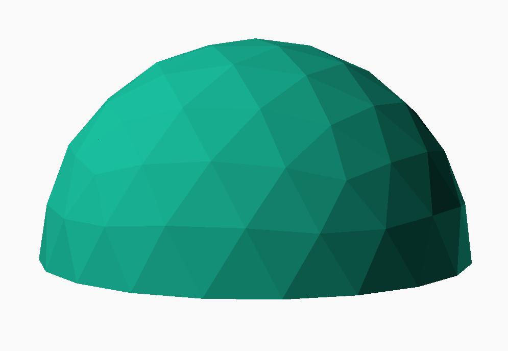

If you have any comments or suggestions to enhance this post or if you’d like to share your experiences with OpenSCAD and geodesic domes, please don’t hesitate to reach out. Your feedback is greatly appreciated, and I look forward to hearing from you!